
Page 172 - Ms Excel Note and Workbook
P. 172
MICROSOFT EXCEL NOTE AND WORKBOOK
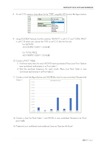
8. At cell C15, create a drop-down list for “TYPE” using the LIST function like figure below.
9. Using VLOOKUP formula, find the matches “MONTH” in cell C17 and “TOTAL PRICE”
in cell C18 when user choose the TYPE at cell C15. Use the formula:
For MONTH:
=VLOOKUP(C15,B5:F11,2,FALSE)
For TOTAL PRICE:
=VLOOKUP(C15,B5:F11,5,FALSE)
10. Create a PIVOT TABLE:
i) Find how many items for each MONTH were purchased. Place your Pivot Table in
new worksheet and rename it as Pivot table 1.
ii) Find the purchase frequency for each month. Place your Pivot Table in new
worksheet and rename it as Pivot table 2.
11. Create a chart like figure below and MOVE the chart to new worksheet. Rename it to
Chart 1.
12. Create a chart for Pivot Table 1 and MOVE to new worksheet. Rename it as Chart
pivot table.
13. Protected your worksheet and workbook. Save as “Exercise Ms Excel”
163 | P a g e